MESA output#
Output files#
By default, MESA stores its data in the LOGS directory. The data files are text-based and can be fed into your favorite plotting program. You should visit the Add-ons section of the MESA forum and see if someone has contributed code in your language of choice. (There are reasonably mature routines for Python, IDL, ruby and Mathematica.) An example of Python plotting is shown later on this page.
In the LOGS directory, you’ll find the following files.
history.data#
The history for the run is saved, one line per logged model, in the file “history.data”. The first line of history.data has column numbers, the second line has column names, and the following lines have the corresponding values. In case of a restart, lines are not removed from the history.data; instead new values are simply appended to the end of the file. As a result the model_numbers are not guaranteed to be monotonically increasing in the log. The code that uses the history must bear the burden of removing lines that have been made obsolete. This can most easily be done by storing the data into arrays as it is read using the model_number as the array index. That way you’ll automatically discard obsolete values by overwriting them with the newer ones that appear later in the history file.
profiles.index#
MESA doesn’t store profiles for every step (that’d take up too much space). This list tells you how to translate between the numbers in the profile filenames and the MESA model numbers. By default, MESA will store a profile at the end of the run.
For each profile, there is a line in profiles.index giving the model number, its priority, and its profile number. Priority level 2 is for models saved because of some special event in the evolution such as the onset of helium burning. Priority level 1 is for models saved because the number of models since the most recent profile has reached the currently setting of the profile_interval parameter.
profile.data#
The profiles contain detailed information about a selected set of models, one model per file. The name of the profile data file is determined by the profile number. For example, if the profile number is 15, the profile data will be found in the file named ‘profile15.data’.
Each profile includes both a set of global properties of the star, such as its age, and a large set of properties for each point in the model of the star given one line per point. In each case, the lines of data are preceded by a line with column numbers and a line with column names.
Selecting output quantities#
The default MESA output is set by the files
$MESA_DIR/star/defaults/history_columns.list
$MESA_DIR/star/defaults/profile_columns.list
In order to customize the output, copy these files to your work directory
cp $MESA_DIR/star/defaults/history_columns.list .
cp $MESA_DIR/star/defaults/profile_columns.list .
Then, open up history_columns.list or profile_columns.list in a text editor. The file describes the full list of the available options. To add/remove the columns of interest, comment/uncomment any lines (‘!’ is the comment character).
But what if you want a history or profile quantity that isn’t on the list? For that, you’ll want to use run_star_extras.f.
Plotting MESA output#
While pgstar is great for observing your stellar models evolving in real time and for quickly making videos, more complicated and higher-quality plots require post-processing in another environment. Perhaps the most popular environment in recent years is Python, and in particular, via the numpy and matplotlib packages.
While you may want to write your own tools to read and analyze the
output of your MESA calculations, many already
exist. In that
vein, we introduce a simple module for use in Python scripts and
interactive sessions called mesa_reader, which only requires
numpy.
What is MESA Reader?#
mesa_reader is a module consisting of three classes that you can use
to read in the contents of a typical LOGS directory. These three
classes are called MesaData, which corresponds to data in profiles
or history files, MesaProfileIndex, which corresponds to data found
in profiles.index, and MesaLogDir, which ties together data in
profiles, the profile index, and the history file.
Full documentation for how MESA Reader is installed and how to use the
three classes can be found at the project’s GitHub
repository and
accompanying
documentation.
How to install MESA Reader?#
The most stable release of mesa_reader can be installed through pip via
pip install mesa_reader
Examples#
Below, we show some simple example use cases of MESA Reader.
The Basics#
# import mesa_reader to make its classes accessible
import mesa_reader as mr

# make a MesaData object from a history file
h = mr.MesaData('LOGS/history.data')

# extract the star_age column of data
ages = h.data('star_age')

# or do it more succinctly
ages = h.star_age
here, ages is now a numpy array that has the same values as are in
our LOGS/history.data file under the star_age header.
That’s how to set up a history file, but what about profiles? We can do the same thing if we know the exact file we want to load:
import mesa_reader as mr

# load the profile file into a MesaData instance
p = mr.MesaData('LOGS/profile1.data')

# access the temperature column of data
temperatures = 10 ** p.logT
But often it’s frustrating to know exactly what profile file you want to
load, so we can use the MesaLogDir class to simplify the process. It
lets us load profiles by their associated model number, or most simply
by just loading the last saved profile:
import mesa_reader as mr

l = mr.MesaLogDir('./LOGS')

# load the profile associated with model number 100
p_100 = l.profile_data(100)
# the same as the following
p_100 = l.profile_data(model_number=100)

# load the profile with PROFILE number 12
p_12 = l.profile_data(profile_number=12)

# load the last profile saved (largest model number)
p_last = l.profile_data()
There are many ways to get at specific profile files and even to select profiles based on criteria in the history file. See the full documentation for more.
An HR Diagram#
Okay, how about making a plot with this data? MESA Reader has no implicit plotting capabilities, but it makes plotting in other environments dead simple. For this example, we’ll use matplotlib and assume that it is being used in pylab’s interactive mode:
# start pylab mode
%pylab
# import mesa_reader
import mesa_reader as mr

# load and plot data
h = mr.MesaData('LOGS/history.data')
plot(h.log_Teff, h.log_L)

# set axis labels
xlabel('log Effective Temperature')
ylabel('log Luminosity')

# invert the x-axis
plt.gca().invert_xaxis()
For an example run simulating a massive pulsating star, this produces something like the following image:
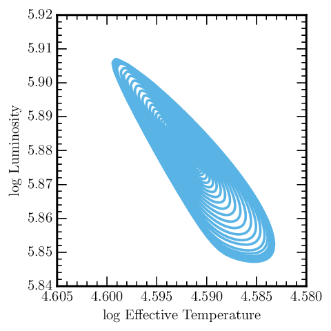
Don’t worry if your plot has a different style than this, as that is
just a function of your matplotlibrc file, which won’t be discussed
here.
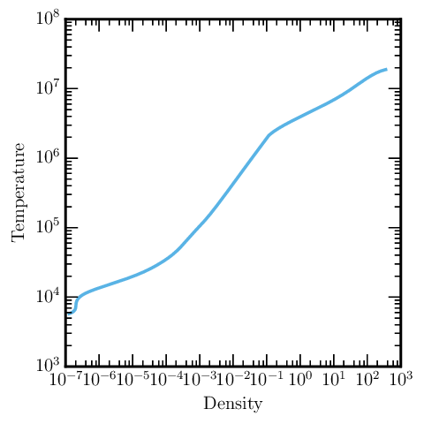
A Temperature-Density Profile#
To plot a temperature-density profile, the process is very similar:
%pylab
import mesa_reader as mr

# load entire LOG directory information
l = mr.MesaLogDir('./LOGS')
# grab the last profile
p = l.profile_data()

# this works even if you only have logRho and logT!
loglog(p.Rho, p.T)
xlabel("Density")
ylabel("Temperature")
which produces something like the following image:
Going Beyond#
MESA Reader is very general and is not just a tool to extract data columns for simple plotting (though that is perhaps the most obvious use). You can use it to filter through your data, selecting only periods or profiles that are match some criterion (say, profiles that were taken when the star was in a particular region of the HR diagram). More complicated plots can be made, like Kippenhahn diagrams, with a little bit more clever work.